Chapter 5 Final Model
Finally! We are ready for our final model! Now, let’s use our test and train data.
load('adoption.RData')
set.seed(454)
adoption_split <- initial_split(adoption, prop = .7)
adoption_train <- training(adoption_split)
adoption_test <- testing(adoption_split)
5.1 Model Building
\[\text{Let }y^*\text{ be the latent variable, }\zeta\text{ be the vector with 2 cutpoints, and }Y_i\text{ be the } \\\text{ ordinal outcome for the ith animal with 3 possible adoption speeds.}\] \[Y_i|\zeta_1,\zeta_2,\beta_1,...,\beta_{16} = \left\{ \begin{array}{ll} 1 & \quad y^* < \zeta_1 \\ 2 & \quad \zeta_1 \leq y^* < \zeta_2 \\ 3 & \quad \zeta_2 \leq y^* \end{array} \right.\] \[y^*=\beta_1x_1...+\beta_{10}x_{10}+\beta_{11}x_1*x_10+\beta_{12}x_2*x_5+...+\beta_{16}x_2*x_9\] where \(x_n\) for n from 1 to 10 is the indicator for cat, minor/severe injury, sterilization, age groups 1-5, and Mix breed.\(\beta_{11}\) is the coefficient for the interaction term of \(Type*MixedBreed\), and \(\beta_{12}\) to \(\beta_{16}\) are the coefficients for the interaction terms of \(AgeGroup*Sterilization\). \[\\\zeta_1 \sim N(m_{01},s_{01}^2) \\... \\\beta_1 \sim N(m_1,s_1^2) \\...\]
5.2 Diagnostic Plots
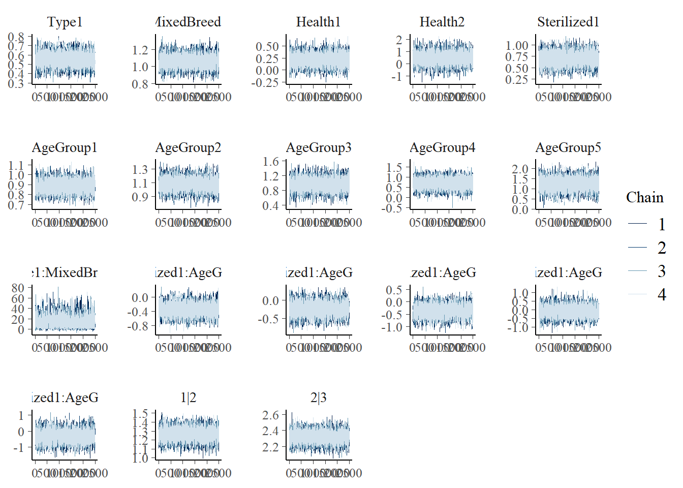
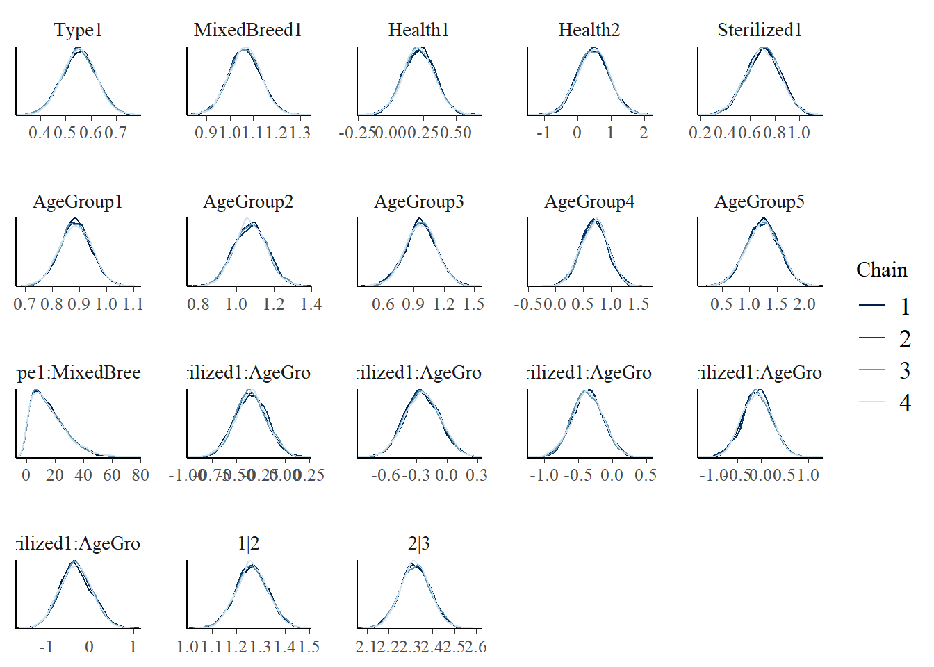
Let’s look at some diagnostic plots! All of these plots don’t show any abnormal pattern and the chains overlap with each other.


5.3 Posterior Inference
##                              mean         mcse           sd         10%
## Type1                  0.55324562 5.450454e-04  0.067972248  0.46483044
## MixedBreed1            1.06318355 6.057704e-04  0.069597623  0.97480407
## Health1                0.21518841 1.110681e-03  0.122186905  0.06095336
## Health2                0.46906848 4.657286e-03  0.485278981 -0.15002129
## Sterilized1            0.70538087 1.342419e-03  0.140259684  0.52140574
## AgeGroup1              0.88612023 5.265084e-04  0.059696574  0.80957865
## AgeGroup2              1.07574108 8.196934e-04  0.087154667  0.96498714
## AgeGroup3              0.97119919 1.484276e-03  0.160364847  0.76596417
## AgeGroup4              0.69497692 2.420120e-03  0.245471775  0.38302011
## AgeGroup5              1.23313469 2.739425e-03  0.301253163  0.84356176
## Type1:MixedBreed1     16.38712159 2.788769e-01 12.224207824  3.10183396
## Sterilized1:AgeGroup1 -0.34854266 1.592412e-03  0.166436814 -0.56054245
## Sterilized1:AgeGroup2 -0.24287677 1.695753e-03  0.174026062 -0.46464188
## Sterilized1:AgeGroup3 -0.36499681 2.226908e-03  0.231066947 -0.65942334
## Sterilized1:AgeGroup4 -0.08299334 3.264202e-03  0.321884568 -0.49697579
## Sterilized1:AgeGroup5 -0.32553321 3.801849e-03  0.381588876 -0.81327658
## 1|2                    1.26453439 5.979261e-04  0.068066142  1.17738499
## 2|3                    2.32111604 6.076589e-04  0.071312780  2.22969547
## mean_PPD:1             0.51028151 7.234882e-05  0.007008311  0.50135325
## mean_PPD:2             0.22274171 5.927455e-05  0.006181765  0.21489661
##                              50%         90% n_eff      Rhat
## Type1                  0.5533768  0.64007248 15552 0.9996826
## MixedBreed1            1.0631939  1.15079427 13200 0.9997197
## Health1                0.2147546  0.36975078 12102 0.9999215
## Health2                0.4669237  1.08419208 10857 0.9998238
## Sterilized1            0.7071647  0.88462549 10917 1.0003414
## AgeGroup1              0.8856529  0.96257346 12855 0.9997073
## AgeGroup2              1.0755650  1.18602234 11305 0.9997492
## AgeGroup3              0.9709156  1.17491749 11673 0.9997387
## AgeGroup4              0.6991856  1.00797587 10288 0.9999504
## AgeGroup5              1.2372309  1.61889575 12093 0.9997890
## Type1:MixedBreed1     13.8552125 33.40589650  1921 1.0013566
## Sterilized1:AgeGroup1 -0.3501312 -0.13333359 10924 0.9999779
## Sterilized1:AgeGroup2 -0.2457145 -0.02067051 10532 1.0000624
## Sterilized1:AgeGroup3 -0.3655172 -0.06871630 10766 0.9999318
## Sterilized1:AgeGroup4 -0.0837725  0.32655525  9724 0.9998016
## Sterilized1:AgeGroup5 -0.3358608  0.17423792 10074 0.9998414
## 1|2                    1.2637562  1.35222578 12959 0.9997043
## 2|3                    2.3203994  2.41246188 13773 0.9996658
## mean_PPD:1             0.5103389  0.51921620  9383 0.9998999
## mean_PPD:2 0.2227996 0.23048609 10876 1.0001687set.seed(454)
model_data<-adoption_test %>%
dplyr::select(AdoptionSpeed_Group,Type,Health,AgeGroup,MixedBreed,Sterilized) %>%
na.omit()
final_prediction <- posterior_predict(
final_model,
newdata = model_data)
ordinal_accuracy2(final_prediction,model_data)## [1] 0.5531591ordinal_predictions<-function(post_preds,mydata){
post_preds<-as.data.frame(post_preds)
results<-c()
for (j in (1:length(post_preds))){
results[j]<-as.numeric(tail(names(sort(table(post_preds[,j]))))[3])
}
results<-as.data.frame(results)
compare<-cbind(results,mydata$AdoptionSpeed_Group)
compare<-compare %>%mutate(results=as.numeric(results))
compare<-compare %>% mutate(`mydata$AdoptionSpeed_Group`=as.numeric(`mydata$AdoptionSpeed_Group`))
compare<-compare %>%mutate(accuracy=ifelse(as.numeric(results)==as.numeric(`mydata$AdoptionSpeed_Group`),1,0))
compare<-compare %>% mutate(pred=ifelse(accuracy==1,as.numeric(`mydata$AdoptionSpeed_Group`),0))
compare %>% count(pred)
}## # A tibble: 3 x 2
## pred n
## <dbl> <int>
## 1 0 1761
## 2 1 1791
## 3 3 389## # A tibble: 3 x 2
## AdoptionSpeed_Group n
## <fct> <int>
## 1 1 2017
## 2 2 923
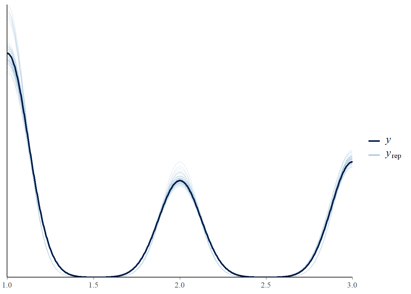
## 3 3 1001Our final accuracy is 55.3%. We can see that our model successfully predicts most of the animals in “Adoption Speed 1”, about 1/3 of the animals in “Adoption Speed 3”, and did not predict any for “Adoption Speed 2”. This could be partially attributable to the fact that we have more animals in group 1. While the expected value of the cofficient for \(Type*MixedBreed\) is 16.4, the standard deviation is fairly large, demonstrating that the variable might be not as significant. The expected value of the cofficient for \(sterilized*AgeGroup\) are more significant for animals in agegroup 1 and 2. If an animal is in age group1 and sterilized, then \(y^*\) will decrease by 0.35, making it more likely to get adopted faster than an animal that is not sterilized and not in age group 1, keeping all other variables constant.
5.4 Discussion
Our model demonstrates that an animal’s health status, sterilization records, age, type (dog/cat), and whether it’s a mixed breed dog or are the factors that are most indicative of the animal’s adoption speed. Our model doesn’t have the most ideal accuracy, and I think this could be attributable to the fact that pet adoption is a rather personal process that varies for each person and animal. For future models, it would be helpful to see if we can downsample when modeling, this might raise the accuracy for “Adoption Speed 2”. One variable that I think can help improve this model is a score of the animal’s appearance. The cuteness/attractiveness of the animal probably plays an important role in the animal adoption process. I noticed that “Mixed Breed” dogs are more likely to get adopted slower, and I this might be due to the fact that theyir appearance are less cute/attractive than pure breed dogs.